What Does an Economic Impact Multiplier Actually Measure?

Economic impact studies often report headline figures that look surprising at first glance. A facility employing 500 people may be said to support 800 jobs across a regional economy. Or $100 million in direct activity may be associated with $165 million in total activity.

Where do the additional jobs and dollars come from?

The answer is the economic multiplier. Multipliers appear in studies of businesses, universities, hospitals, tourism, infrastructure, data centers, nonprofits, and many other kinds of activity. They are also among the easiest parts of an impact study to misunderstand.

The basic idea is simple: a business does not operate alone. It buys from other businesses; those suppliers employ workers and make purchases of their own; workers then spend some of their income locally. A multiplier is a way of tracing those relationships while recognizing that a portion of each spending round leaves the region.

Start with the Direct Effect

Suppose a company opens a facility and employs 100 people. Those 100 positions are the direct jobs. If the facility produces $20 million of output, that is direct output. If it pays $7 million in wages and benefits, that compensation is part of the direct activity associated with the facility.

Nothing has been multiplied yet.

The next question is what the company needs in order to operate. It may purchase electricity, maintenance, accounting, transportation, security, equipment, professional services, and many other inputs. Some purchases come from businesses located within the study area. That is where the additional layers of activity begin.

Local Suppliers Create Indirect Effects

Economists call the supply-chain response the indirect effect. Suppose the company purchases $2 million of goods and services from local suppliers. Those suppliers employ workers and purchase inputs themselves. A maintenance contractor buys equipment; a transportation company pays for repairs; an accounting firm purchases software and office services.

The spending works its way through the regional supply chain, but each round becomes smaller. Equipment may come from another state. Software may be purchased from a national company. Firms pay taxes, save part of their income, and distribute profits that may leave the study area. These are examples of leakages—money that does not continue circulating within the region.

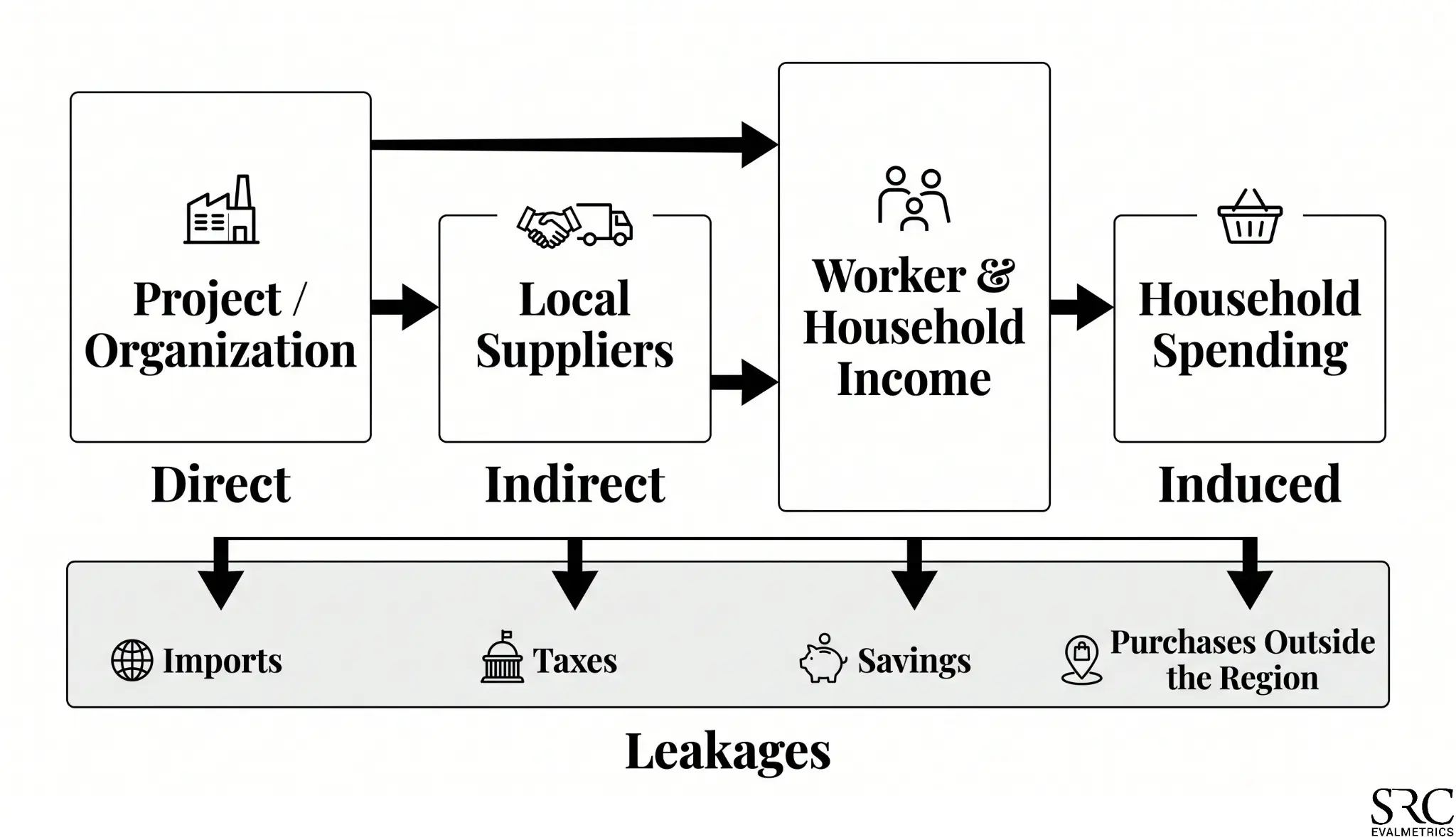
Geography therefore matters enormously. A county has a smaller supplier base than an entire state. A firm operating in a county may need to buy many inputs elsewhere; if the study area expands to the state, some of those purchases may now count as local. The same project can consequently have a larger multiplier at the state level than at the county level. That is not a contradiction—the definition of “local” has changed.

Workers Create Induced Effects

There is another channel. The company pays its workers, and its local suppliers pay their workers. Those households spend part of their income on groceries, housing, restaurants, health care, transportation, entertainment, and other goods and services. When that spending occurs within the region, it supports additional jobs and income.

Economists call this the induced effect.

Induced spending does not occur only after the supplier effect. Workers at both the original organization and its suppliers receive income. A better way to picture the process is that direct activity and indirect activity both generate household income, which then produces induced spending.

What a Multiplier of 1.8 Actually Means

Suppose an industry has an output multiplier of 1.80. If a project generates $10 million in direct output, the model estimates:

$10 million × 1.80 = $18 million in total regional output

The first $10 million is the direct effect. The additional $8 million represents estimated indirect and induced activity associated with local supply chains and household spending.

This does not mean that the original $10 million somehow became $18 million in new wealth. Output measures economic transactions. One company’s purchase can become another company’s sale, so output includes intermediate transactions between businesses. For many questions, value added is more useful because it is conceptually comparable to GDP and removes the value of intermediate inputs.

Employment, labor income, value added, and output also have different multipliers. An output multiplier should not be applied to jobs, and an employment multiplier should not be applied to dollars of output. These distinctions may sound basic, but they matter when interpreting an economic impact study.

Type I and Type II Multipliers

Readers may also encounter Type I and Type II multipliers.

• Type I generally captures direct plus indirect effects.
• Type II adds induced effects: direct, indirect, and induced activity.

Modern economic impact systems can use more detailed household and social-accounting structures, so exact treatment varies by model. The intuition is the same: once induced effects are included, worker income becomes another channel through which economic activity can circulate locally.

Where Multipliers Come From

Multipliers can appear to be proprietary numbers that emerge from a black box. The basic economic structure behind them is not mysterious.

Industries buy inputs from other industries. The U.S. Bureau of Economic Analysis publishes national Input-Output Accounts describing these relationships. One industry buys electricity; another purchases transportation services; manufacturers purchase materials and professional services; hospitals purchase medical supplies, utilities, food, insurance, and other inputs.

Economists convert these relationships into a technical coefficient matrix, which describes the inputs required to produce a dollar of output in each industry. Standard input-output mathematics can then estimate not only the first round of purchases, but later rounds as suppliers purchase from their own suppliers.

The harder problem is regionalization.

Ohio Is Not the United States, and Franklin County Is Not Ohio

A national input-output table can describe how much transportation, professional services, machinery, or agricultural inputs an industry typically purchases. A study for Franklin County must answer a more specific question: how much of that demand can actually be supplied from within Franklin County?

Anything that cannot be supplied locally becomes leakage. Commercial systems such as RIMS II and IMPLAN use regional economic information to estimate these local purchasing relationships. That is a major reason multipliers differ across locations.

A manufacturing multiplier estimated for Ohio is not automatically appropriate for Franklin County, rural Wyoming, or metropolitan Chicago. The underlying economies are different.

Can We Recreate Multipliers Using Public Data?

That question motivated my recent working paper, Reproducible Regional Multipliers from Public Data: Benchmarking a Public-Data FLQ Model Against RIMS II and IMPLAN.

The practical question was straightforward: how closely can commonly used commercial multipliers be approximated using data that anyone can download? The model uses two public federal datasets—the Bureau of Economic Analysis Input-Output Accounts and Bureau of Labor Statistics Quarterly Census of Employment and Wages (QCEW)—and regionalizes national production relationships using the Flegg Location Quotient (FLQ) method.

If a supplying industry has a strong presence in a region, the model treats the region as more capable of supplying that input locally. If the industry has relatively little presence, a larger share of the purchase is treated as coming from outside the region. Those regional purchasing estimates are then incorporated into the input-output model to calculate multipliers.

I tested the approach for Ohio, Franklin County, and the Columbus metropolitan area, then compared the public-data results with commercial estimates from RIMS II and IMPLAN.

What the Research Found

At a broad level, public-data estimates came fairly close. For Ohio, aggregated into 15 broad sectors, the public-data model’s Type II output multipliers differed from RIMS II by an average of 8.8 percent and from IMPLAN by 10.9 percent. For comparison, RIMS II and IMPLAN differed from one another by 8.4 percent.

There is no directly observable “true multiplier” sitting in the economy against which every model can be judged. RIMS II and IMPLAN use different regionalization methods and modeling choices, so their estimates differ as well. At the broad sector level, the public-data model was roughly as close to the commercial systems as the commercial systems were to one another.

Using a parameter value from the FLQ literature, a fully public-data version produced average errors of roughly 11 percent relative to RIMS II and 12 percent relative to IMPLAN across the three regions. For preliminary analysis, classroom work, small nonprofits, local agencies, or researchers who need broad-sector estimates, that result is useful. It also makes the multiplier less of a black box.

Where the Public-Data Approach Becomes Less Reliable

The results changed substantially when the analysis moved from broad sectors to detailed industries. At roughly 400-industry detail, the public-data model did a much poorer job reproducing the pattern of commercial multipliers. Some of the largest errors appeared in agriculture, food processing, dairy, oilseed processing, animal feed, and related industries.

The reason makes economic sense: employment is not always a good proxy for production. Agriculture, energy, utilities, and other capital-intensive industries can produce large amounts of output with relatively few workers. An employment-based regionalization method can therefore conclude that a region has little supply capacity even where substantial production occurs.

The boundary is clear. A public-data method can provide reasonable broad-sector estimates; it is less reliable when analysis depends on detailed industry-specific supply chains. For that work, the regional trade information in systems such as IMPLAN and RIMS II remains valuable.

The Multiplier May Not Be the Biggest Source of Error

Analysts can spend considerable time debating whether the right multiplier is 1.6, 1.7, or 1.8. Sometimes that difference matters. But a larger error can occur before the multiplier is ever applied.

Suppose a study begins with $100 million of “direct spending,” but only $60 million represents genuinely new spending in the region. A sophisticated multiplier applied to the wrong $100 million does not fix the problem; it carries the original error through the rest of the model.

The direct effect has to make economic sense first. What spending is truly new to the region? Where does it occur? Which workers are actually associated with the project? Is the activity temporary or recurring? What geography is appropriate? Are we measuring economic activity or economic benefit?

A multiplier is a useful tool, but it is not the economic impact itself. It traces the connections between a project, suppliers, workers, and households while recognizing that part of each spending round leaves the region. My recent research suggests that a surprising amount of that broad structure can be recreated from public data. It also identifies where that approach stops being dependable.

References

Roychoudhury, S. (2026). Reproducible Regional Multipliers from Public Data: Benchmarking a Public-Data FLQ Model Against RIMS II and IMPLAN. Working paper, July 2026. View the paper on SSRN

U.S. Bureau of Economic Analysis. Input-Output Accounts and RIMS II User’s Guide.

U.S. Bureau of Labor Statistics. Quarterly Census of Employment and Wages (QCEW).

Flegg, A. T., & Webber, C. D. (2000). “Regional Size, Regional Specialization and the FLQ Formula.” Regional Studies, 34(6), 563–569.

Miller, R. E., & Blair, P. D. (2009). Input-Output Analysis: Foundations and Extensions (2nd ed.). Cambridge University Press.

Bess, R., & Ambargis, Z. O. (2011). Input-Output Models for Impact Analysis: Suggestions for Practitioners Using RIMS II Multipliers. Bureau of Economic Analysis Working Paper 0081.

IMPLAN Group LLC. IMPLAN Data and Methodology.